Using VLOOKUP to Correlate Data in Microsoft Excel
A practical data tracking reference for using the VLOOKUP function to isolate, map, and merge associated data datasets across separate spreadsheet tables using a common identifier variable.
Consolidating the Target Worksheets
Open the workbook containing your supplemental source data. If the target information resides on a completely separate file, copy all data rows from that sheet and paste them into a brand-new tab within your primary workbook file, then close the external file.
On your primary data spreadsheet worksheet, single-click directly inside the specific cell grid row where you want the final correlated output of the lookup function to be displayed.
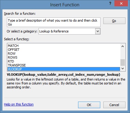
To begin building the syntax, click the Insert Function button (fx) located directly above the main cell matrix area and immediately adjacent to the primary spreadsheet formula bar.

In the "Select a category" dropdown menu subfield, choose Lookup & Reference. From the updated list of available function names below it, scroll down, highlight VLOOKUP, and double-click to load the module interface.
Click inside the Lookup_value input field. This requires a common shared variable present on both worksheet tabs to act as a key index (e.g., names, IDs, years). Click the column letter header on your primary sheet to bind the entire matching reference row array.
Click inside the Table_array input field, then select the tab containing your supplemental background information. Click and drag across the top column letter coordinates to highlight from Column A all the way over to the column holding your desired output target string data.
Click into the Col_index_num input field and type the total integer count of the columns you highlighted in the Table_array step (e.g., if you highlighted columns A through D, your column index value is 4).
Click into the Range_lookup field and type the exact phrase FALSE to command the calculation engine to locate exact value matches exclusively, rather than nearest approximations.
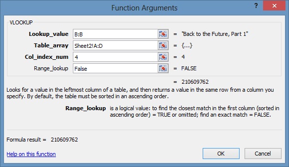
Click OK to finalize and instantiate the formula execution blocks across your grid row coordinates. If mapped cleanly, your target cell will instantly display the matched reference cell data points pulled over from your second worksheet.
To permanently preserve your resolved VLOOKUP data points and safe-delete your secondary data tab without corrupting cells, copy all formula output cells. Right-click the active selection block, select Paste Special, toggle the Values radio choice option parameter, and click OK.